Student Resources - Important Concepts, Terminology, and Numbers
In this section I will attempt to define and/or explain terms that I wish someone had explained to me rather than assume I knew what they meant (principle #2). Developing a working knowledge of these terms and their proper uses will not only allow you to focus more on learning important concepts during your time in the reading room, but it will also help you convey the sense that you've been diligently reading and know what you're talking about, which will in turn make people more willing to teach (principle #1). For many of these terms, seeing is understanding and so when possible I will provide an image as an example. For simplicity's sake, nearly all of these definitions will be over-generalizations, such that there are some restricted circumstances for which they may not apply. They're good enough for 95% of the time, though, and should certainly work for you at this stage. I will focus on general modality topics as well as those in some of the “core areas” of observation. If you encounter a term or a concept during your month with us that you think should be included here for the benefit of future students, please let me know.
“Old films and old reports are a radiologist’s (and a student’s) best friend” – This is an important principle that is worth giving some attention. From the radiologist's standpoint, the idea is that old films and old reports give useful information that can prove invaluable in putting the current examination to be interpreted in an appropriate context and allowing for the most accurate and most clinically useful interpretation to be given. From the medical student's standpoint, the idea is a little different but nonetheless important. At the Brigham and referral centers like it, zebras are rather common, but by the time the patient arrives here, much (if not all) of the workup (including imaging) has already been performed at an outside hospital. While you are practically guaranteed to see imaging of patients with extremely rare disease processes during your month with us, you are far more likely to encounter follow-up or post-treatment imaging of these entities than you are to encounter the initial presentation. To take full advantage of the diverse pathology you will encounter, I urge you to look back at the most interesting patients’ earliest available prior scans, which are most likely to represent the initial presentation and to give you a sense of what these zebras look like before are been identified as such.
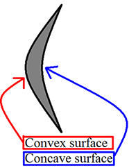
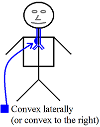
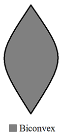
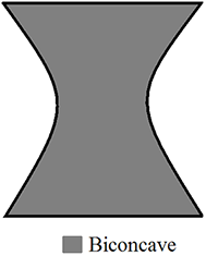
Convex and concave – These terms will be used frequently to describe the margins of structures (lesions or otherwise) and were a source of confusion for me for an embarrassingly long time. You may have these rather simple concepts mastered already, and if so please skip ahead. If you’re like me and want a refresher (or perhaps an introduction), I hope you will find the following diagrams helpful. I frequently must stop to remind myself that “Concave has the cave.”
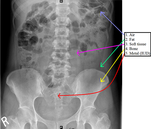
Radiographic opacities – “Opacity” is synonymous with density and can be thought of as “Grayness” in an x-ray image. From a physics standpoint, x-rays pass through the body and “expose” a detector on the opposite side of the patient. When there is tissue between the x-ray source and detector, some of the beams are blocked (“attenuated”) to varying degrees, resulting in differential exposure of the film. Differences in “attenuation” allow us to define 4 elementary densities: air (normally seen in the lung and bowel, but always look for it elsewhere!), fat, soft tissue, and bone. A fifth density that may be seen in some patients is metal.
Oral contrast – Oral contrast is frequently (but not always) given before obtaining CT scans of the abdomen and pelvis. There are two types of oral contrast – barium and Gastrografin (diatrizoic acid). Barium is cheaper and used more frequently, however, it is contraindicated in the setting of suspected perforated viscous, as it can cause peritonitis. Gastrografin is water soluble and should be used in this scenario. Gastrografin is contraindicated in the setting of suspected aspiration, as it can cause severe pneumonitis.
Iodinated IV contrast – Unless contraindicated (due to allergy or renal function), iodine-based IV contrast is typically administered prior to CT exams. Situations in which contrast may be withheld include a patient with hematuria and flank pain (looking for stones) or in unstable patients with suspected acute hemorrhage. Regarding iodinated contrast allergies, if the allergy is considered mild (hives, itching) or moderate (bronchospasm), the patient is typically premedicated with oral steroids prior to the exam. In the case of severe allergy (anaphylaxis), exams with IV contrast are simply not performed.
Iodinated contrast has been associated with acute renal failure in some patient populations (contrast induced nephropathy, CIN, is a term used by some). It is widely believed (by radiologists and non-radiologists) that patients with poor baseline renal function are more susceptible to this phenomenon, however, in recent years, there is much controversy in the medical literature as to whether CIN is as common as once thought (or even if it is real at all!). Practice guidelines are constantly changing (and will likely continue to change) but the current practice at BWH is to use the estimated Glomerular Filtration Rate (eGFR) to determine risk. If the eGFR is >60, the full dose of IV contrast is given and if the eGFR is <30, IV contrast is withheld unless the patient is on hemodialysis. For cases of 30<eGFR<60, the decision to give IV contrast is nuanced and usually requires a patient-specific assessment of risk/benefit.
CT densities – In addition to the densities mentioned above that can be differentiated by radiography (air, fat, soft tissue, bone, and metal), CT allows for the differentiation between soft tissue and fluid by measuring the Hounsfield units (soon to be defined). Compare the measured values given within each ROI (see below for definition) with the expected values listen in the Hounsfield unit (HU) table. Know that values measured in patients may differ slightly from the “ideal” or theoretical values for a number of reasons.
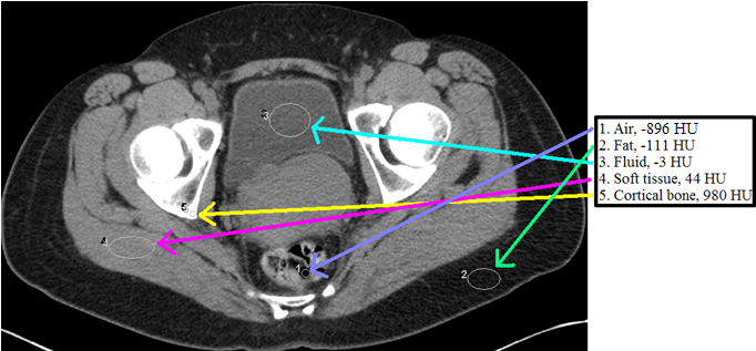
Region of Interest (ROI) – You will likely hear an attending tell a trainee to “Put an ROI on it and see what it is.” ROI stands for region of interest, and this tool is most frequently depicted as an oval on the PACS toolbar. This feature allows you to measure the Hounsfield units of given area on the image, which in turn allows you to better characterize what is going on with the patient.
Hounsfield units (HU) – Sir Godfrey Newbold Hounsfield shared a Nobel Prize for his contributions to developing computed tomography. The Hounsfield unit scale allows for the quantitative representation of CT density. In every day practice this is important because it allows radiologists to select a region of interest (ROI) on a given image and be given the averaged density of that region in Hounsfield units, which subsequently allows for further characterization of a CT finding based on the value given. Common examples of the utility of the Hounsfield unit measurement include determining whether a lesion enhances and whether a fluid collection is likely to be simple or complex. If you look in ten different places, you’ll see ten slightly different characterizations of what Hounsfield units correspond to different tissues. With that in mind, the following table should give you a rough idea of the expected values for some commonly encountered tissues:
| HU | Corresponding Tissue |
| -1000 | Air |
| -120 to -60 | Fat |
| 0 | Water |
| 15 | CSF |
| 30 to 40 | Most soft tissues |
| 35 to 45 | Flowing blood |
| 40 to 60 | Liver |
| 50 to 70 | Acute hemorrhage/acute clot |
| 300 to 400 | Trabecular bone |
| 1000+ | Cortical Bone |
Maximum intensity projection (MIP) – This is a post-processing technique that projects the most intense or brightest data (highest Hounsfield units) from a “slab” (stack of multiple contiguous image slices) onto a single image. This technique is particularly useful for tracing tubular structures such as vessels and for causing non-tubular structures, such as lung nodules, to be more apparent. There are several studies showing that the detection of lung nodules is improved when using this technique.
Minimum intensity projection (MinIP) – This is a similar concept to maximum intensity projection except with this technique the least intense or darkest data (lowest Hounsfield units) is projected. This is used far less frequently but can be helpful for evaluating the airway and other relatively low-density structures.
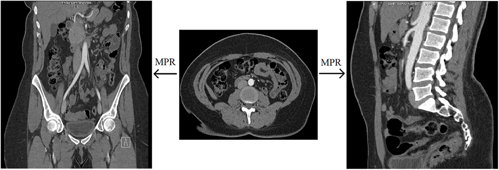
Multiplanar reformat (MPR) – This is a post-processing technique that is simply a more generic way of describing coronal or sagittal projections of axially-acquired CT data. Simply put, coronal and sagittal projections are types of multiplanar reformats.
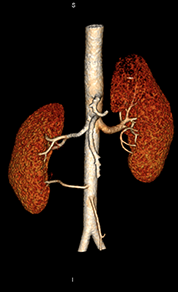
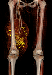
Volume rendering – In radiology, you will hear this term used to describe the post-processing technique used to create the 3D images that surgeons find very useful for preoperative planning. Typically, this type of post-processing is done because the ordering physician finds it helpful and not because radiologists use these images to make diagnoses. For diagnosis, radiologists look to the source images.
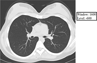
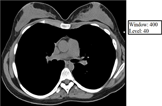
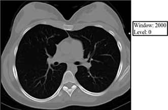
Window and Level – These are two interrelated concepts that are frequently used together as one term and together determine how the numerical Hounsfield units are converted into and displayed as shades of gray on the PACS monitor. As you saw in the Hounsfield unit table above, densities within the human body range over about 2000 HU (air -1000 to bone +1000). If each Hounsfield unit were to correspond to a single shade of gray, you could think of the human body as represented by CT as having as many as 2,000 shades of gray. Generally, the PACS monitors can display about 256 shades of gray, and the human eye can discern even fewer (roughly 15 by most estimates). Thus, if we as human readers are going to glean the maximum amount of information (tissue densities as expressed in Hounsfield units) from a given CT scan, it is necessary that we look at the data in bits and pieces, and the way we divide the data into usable bits and pieces is through appropriately using the window and level functions.
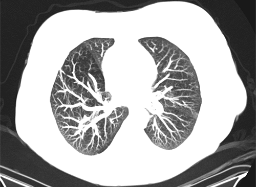
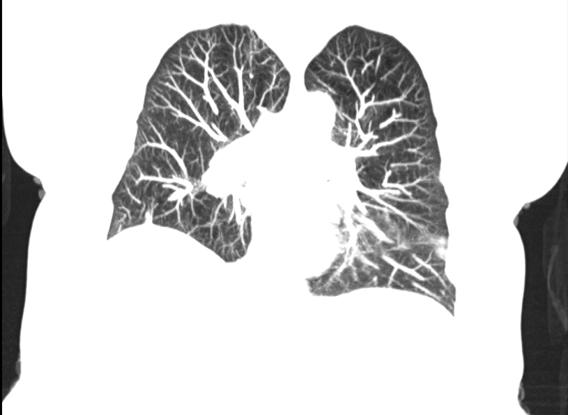
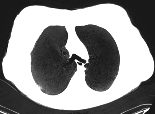
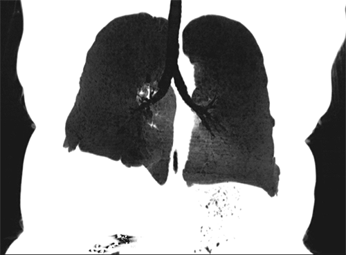
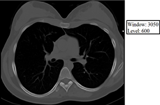
The level value sets the center of the gray scale (think of this as what HU will be displayed as exactly between black and white), and the window value sets the range of Hounsfield units above which everything will be displayed as white, below which everything will be displayed as black, and between which everything else will be assigned various shades of gray as a function of its relationship (bigger or smaller than) the level value. Below are some examples of how changing the window and level alters the image presentation. Given your understanding of Hounsfield units, window, and level, think about why each of the following images appears the way it does. The first 3 images demonstrate lung, soft tissue, and bone windows, respectively. The fourth image is for demonstration only and would generally not be used for diagnostic purposes. Note that it most closely approximates a bone window.
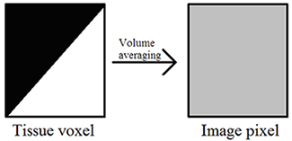
Volume averaging – The unit of acquired CT data is the voxel, and each voxel is displayed on the PACS monitor as one pixel. A single voxel in the human body may have multiple densities corresponding to multiple Hounsfield units, but a single pixel on the PACS monitor must display a single shade of gray corresponding to a single Hounsfield unit. Volume averaging describes the result of the situation in which a portion of a given voxel has one tissue density and another portion of the same voxel has a (oftentimes very) different tissue density. Because the pixel that corresponds to this voxel may only display a single shade of gray corresponding to a single Hounsfield unit value, the densities within the voxel are averaged together, and it is this average that is ultimately displayed within the corresponding pixel on the PACS monitor. Volume averaging is a source of error and is increased by motion.
Hyper/hypodense – With CT, bright tissues appear bright because they are denser than surrounding tissues, and dark tissues appear dark because they are less dense relative to their surroundings. This is the SAME principle we saw with chest x-rays! Therefore, when describing CT images, you should describe bright areas as “hyperdense” and dark areas as “hypodense.” If asked to compare two tissue densities and they appear to you to be the same, say they are “isodense.” The descriptive terms you will use for MRI and US will be different, and though this may seem nitpicky, when used appropriately, it will go a long way toward giving the impression to those around you that you know what you are talking about.
A detailed understanding of MRI is beyond the scope of this clerkship, but you will likely see MR images during your time with us. Thus, it is worth knowing a little bit of background.
Signal – As opposed to CT, where tissue contrast is derived from varying tissue densities, you should know that in MRI, tissue contrast is derived from differences in signal intensity of the protons making up the different tissues. Areas of high proton signal are displayed as bright, while areas of low proton signal are displayed as dark.
Hyper/hypointense – Because it is signal intensity differences that allow you to differentiate different tissues on the MR image, if you wish to describe MR images correctly, it is important that you describe bright areas as “hyperintense” and dark areas as “hypointense.” If asked to compare two tissue intensities and they appear to you to be the same, say they are “isointense.”
Gadolinium contrast – Chelated gadolinium contains seven free electrons, which leads to “T1 shortening” in the physical realm and T1 brightness on the image, and it is for this reason that gadolinium is used as an intravenous MRI contrast agent. Just like with iodinated CT contrast, there are also contraindications to gadolinium, and, also like CT contrast, they have to do with patient allergies and patient renal function. Allergies to gadolinium are rarer than allergies to iodinated contrast, but they do occur and are treated similarly, with patients with mild to moderate reactions being pretreated with corticosteroids and patients with severe reactions (anaphylaxis) not receiving any gadolinium with future exams. With regard to renal function, we again base our decision to give or withhold IV contrast based on the patient’s eGFR, but with gadolinium, it’s “all or nothing” (there is no reduced dose), and our reason for caring about the patient’s renal function is not because gadolinium is thought to have an adverse effect on the kidneys. For gadolinium contrast, we give the full dose to anyone with an eGFR greater than 30, and for a eGFR less than or equal to 30, we withhold gadolinium (regardless of whether the patient is receiving hemodialysis) out of concern that s/he may develop nephrogenic systemic fibrosis.
Nephrogenic systemic fibrosis (NSF) – Nephrogenic systemic fibrosis is a debilitating and ultimately fatal disease that has been shown to develop in patients with poor renal function (all reported cases had eGFR<30 at the time of the scan) who receive IV gadolinium contrast. The first cases were described in 1997, and the condition involves fibrosis of the skin and internal organs. Even in patients with poor kidney function, NSF is exceedingly rare. However, because it is so debilitating and ultimately fatal, even the very small risk of doing this to a patient is considered to be too great to give gadolinium in this population.
T1 and T2 – You will (if you have not already) undoubtedly hear about T1 and T2 in the context of MRI on this rotation. Again, a detailed understanding is far beyond the scope of this clerkship, but it is worth knowing that both T1 and T2 represent times (on the order of ms). A given tissue will have both a T1 and a T2, and as a general rule T2 is shorter than T1 for all tissues. T1 has to do with protons regaining their longitudinal magnetization, while T2 has to do with protons losing their transverse magnetization. For the interested student, you have been given some terminology that you may now read more about (the RSNA physics modules are good but require registering as a member). For those of you who may not be interested in MR physics (and kudos to you), feel free to remember that T1 and T2 are both times and forget everything else mentioned in this paragraph.
Hyper/hypoechoic – Unlike CT and MRI, where tissue density and tissue proton signal are measured and subsequently provide image contrast, with ultrasound it is the tendency of different tissues to reflect and absorb sound waves to a different degree that allows for tissue contrast on the generated image. Bright tissues on the image reflect more sound waves and should therefore be described as “hyperechoic.” If a structure reflects no sound waves back, it will be completely black on the image and should be described as “anechoic.” (“without echoes”). If the structure reflects few sound waves back it will be dark but not completely black, and in this case you should call it “hypoechoic.” When two different structures have the same echogenicity, say they are “isoechoic.”
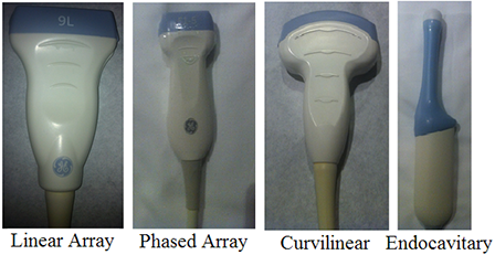
Probe selection – In an attempt to skirt a prolonged discussion of the underlying (and for your purposes largely unnecessary) physics, let’s focus on the more practical clinical decision of “Which probe do I pick up to scan the patient?” The (high frequency) linear array probe is good for seeing superficial structures in great detail (think high frequency = high resolution, poor penetration). The thyroid, the breast, and superficial vessels are frequently imaged with this probe. The medium frequency phased array probe allows you to look a little deeper at the cost of some resolution, and this probe is most commonly used in echocardiography. The low frequency curvilinear array probe gives you the most penetration but also the lowest resolution (low frequency = low resolution, good penetration). This probe is generally used to image deeper structures in the abdomen and pelvis. The endocavitary probe has a curved surface like the low frequency curvilinear probe but images at high frequencies to give better resolution. The poorly penetrating sound waves are acceptable because of the placement of the probe in close proximity to the anatomic area of interest. This probe is most commonly used in obstetric and gynecologic imaging. Probe photos courtesy of Asha Sarma, MD.
Doppler – The Doppler function on ultrasound allows for the detection of flow. There are different types of Doppler ultrasound, which you will likely learn about later in the rotation. Doppler ultrasound takes advantage of the subtle apparent frequency change that takes place in a sound wave when it reflects off of a moving object (Doppler effect). In the case of medical imaging, the moving object is flowing blood. Often, the flow velocity can be estimated, as it is proportional to the amount of observed frequency change. There are many applications of Doppler ultrasound in medical imaging, but common ones include assessing for vascular thrombus or stenosis and characterizing the vascularity of an abnormal (or normal in the case of torsion) structure.
There are a number of ultrasound (and other imaging modality) artifacts that a radiologist must be able to recognize to appreciate the limitations of a study and to avoid wrongly diagnosing apparent pathology that is actually artifact. We will leave these types of artifacts to the radiologist. There are additionally some ultrasound artifacts that, when present, actually help you make a diagnosis, and for this reason are worth covering here. Once you see these, you’ll never forget them.
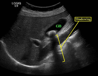
Shadowing – Shadowing describes the situation in which whatever is deep to an intense reflector (typically a stone) appears falsely hypoechoic or even anechoic. Shadowing artifact, when present, is then helpful in differentiating stones from other nonspecific hyperechoic foci.
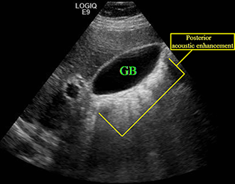
Posterior acoustic enhancement (increased through transmission) – In contrast to shadowing, posterior acoustic enhancement or increased through transmission describes the situation in which whatever is deep to a poor reflector (typically fluid) appears falsely hyperechoic. Posterior acoustic enhancement is a characteristic of a simple cyst, but it can be seen in other entities. The example provided here shows increased through transmission posterior to the gallbladder.
Twinkle – Twinkle artifact describes the situation in which rapidly alternating red and blue is seen in Doppler mode and most commonly happens in the setting of a strong reflector with rough surfaces, such as a stone. Twinkle may be seen in a number of circumstances, including adenomyomatosis of the gallbladder, cholelithiasis, nephrolithiasis, and chronic pancreatitis, however, it can be most helpful for detecting and differentiating small ureteral stones from other nonspecific hyperechoic foci. This is very difficult to demonstrate with a single static image, but it is something you will observe the sonographers looking for in their patients.
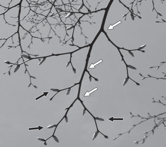
“Tree-in-bud” opacity – If you think of this as “budding tree” or “tree with buds” opacity, you may find it a lot easier, and this is another example of seeing equating to understanding. “Tree in bud” opacities are typically seen in the setting of alveolar disease processes.
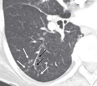
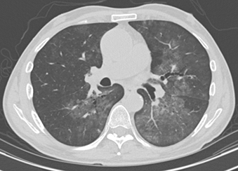
Groundglass opacity – Groundglass opacity describes the finding of increased lung attenuation to the point that it appears hazy but not to the point that the vessels coursing through that area of the lung are obscured. This is a nonspecific finding seen in a variety of settings, but a reasonable differential could include pulmonary edema, pulmonary hemorrhage, PCP pneumonia, and hypersensitivity pneumonitis. In the example below, note that the vessels can be distinctly seen within the left greater than right hazy opacity (the patient’s left).
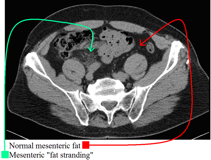
Fat stranding – Fat stranding describes the nonspecific increased attenuation (“schmutz” or “dirty fat”) of the local fatty tissues that is frequently seen in the setting of an adjacent acute inflammatory processes. This term is ubiquitous in radiology reports, so try to learn what it looks like from day 1! Histologically, fat stranding represents edema/fluid infiltrating fatty tissue. As you recall, fat typically has a nearly black appearance on CT (-120 to -60 Hounsfield Units) whereas water/edema are gray (0 Hounsfield units): when edema is present within fat (fat + water volume average = (-60 + 0)/2 = -30, it will become hazy/gray, often in a linear (perilymphovascular) pattern hence the term “stranding of the fat”. When you think of the cardinal signs of inflammation (tumor, rubor, dolor, calor), this is the radiographic equivalent of “tumor” or swelling! This can help to localize pathology i.e. in appendicitis, you see peri-appendiceal fat stranding; in diverticulitis you frequently see peri-diverticular fat stranding, and in pancreatitis you frequently see fat stranding surrounding the pancreas. In this case, the patient’s dilated, inflamed appendix was seen a few slices inferiorly.
Incidentaloma – This term is often used to refer to an incidental mass. An incidental finding is one that is unrelated to the clinical indication for the imaging exam performed. These “incidentalomas” are frequently encountered and, depending on their location, are usually benign (renal cysts, adrenal adenomas). However, even likely benign lesions can prove problematic (RCC can be cystic and adrenal nodules can represent metastases). You will likely notice that the description of these findings and recommendations for possible further evaluation will vary from radiologist to radiologist.
Some numbers – Upper limits of normal and other numeric values are notoriously variable and you will no doubt hear other values for some if not all of these, however, the following is a list I have compiled that will at least give you a ballpark idea. I have attempted to list these in order of likelihood that you would be expected to know them. This is meant more to give you a general idea than to be memorized, and truthfully if you know ANY of these, your resident and attending are likely to be impressed.
| Region of Interest | Measurement |
| Appendix diameter | 6 mm (if greater, consider dilated) |
| Gallbladder wall | 3 mm (if greater, consider thickened) |
| Gallbladder lumen | 2-5 cm (if <2, contracted; if >5, distended) |
| Kidney stone | 6 mm or smaller likely to pass spontaneously; larger likely to need intervention |
| Common bile duct | 5-7 mm (can depend on age so in elderly patients 8mm or greater could be normal) |
| Small bowel lumen | 3 cm |
| Small bowel wall | 3 mm |
| Colon lumen | 5 cm |
| Colon wall | 5 mm |
| Cecum lumen | 8 cm |
| Prostate | 4 cm |
| Spleen | enlarged if >14 cm in any dimension |
| Bladder wall | 6 mm |
| Adrenal limb thickness | 5-7 mm |
| Pancreatic duct | 3-4 mm |